
Build Your Own Static Vector Tile Pipeline
James GardnerFollowing on from James Milner’s introduction to Tiler, this post will drill into a little bit more detail about vector tiles, and the low-level commands tools like Tiler use behind the scenes. By understanding the commands, you’ll be able to build your own static vector tile pipeline.
NOTE: If you want to generate vector tiles that frequently need updating, you would be better off importing your data into PostGIS and then using a tool such as Tegola to generate them dynamically from the database as they are requested. The approach described in this post is better for generating a set of vector tiles all in one go.
This post describes the exact commands you’ll need to run assuming you are on the latest macOS (the most common set up amongst Engineers at the Hub at the moment). The same pipeline will work on Linux as well as previous versions of MacOS if you install the core tools we use yourself.
We’ll also assume you have a basic geospatial knowledge. If you haven’t, it is worth knowing that shapefiles, GeoJSON and TopoJSON are just ways of storing points, lines and areas. Within each file, each point, line or area is called a feature. Web maps generally load the data they need to display in tiles, small squares of data that each represent one small part of the map you are looking at.
Read this GIS File Formats page first for an overview of different approaches and their pros and cons.
It is also worth knowing that, slightly confusingly, a single shapefile is
actually distributed as four separate files, and that you need all four to be
able to work with the shapefile, not just the .shp file itself.
Throughout this tutorial we’ll be using compressed vector tiles that are smaller to store and quicker to transfer than their uncompressed counterparts.
Also, if you stop the tutorial and pick it up again, you’ll need to re-run all
the export commands to set up all your paths correctly again.
Mapbox Vector Tiles
Mapbox Vector Tiles are a modern way of storing and transmitting the same sort of feature data you might ordinarily find in a shapefile, GeoJSON or TopoJSON file.
There are two features of vector tiles that make them particularly interesting as a source format for displaying data on maps:
- In preparing the tiles, the data for the features the tileset represents is chopped up into individual tiles. This means the data for a large feature like a coastline will no longer exist as a single complex shape, but instead each tile that needs to display a portion of it will contain just the information needed to render the part of the coastline it is responsible for.
- Mapbox Vector Tiles are a compact binary encoding of the vector data called Google Protocol Buffers that is smaller than corresponding JSON, and usually smaller than a corresponding traditional raster tile too.
Because of these innovations, vector tiles have a major advantage over non-tiled formats like GeoJSON and TopoJSON:
- Map clients only need to download the data for the tiles they need to display, not all the data for all features that have some part on the map (as they would with GeoJSON or TopoJSON)
- Even if source GeoJSON or TopoJSON was prepared as separate tiles, Vector tiles can be obtained by browsers more quickly because they are a more compact binary format so file sizes are lower.
Being a vector format (containing portions of the actual source data), vector tiles have advantages over traditional raster tiles (just pictures of the pre-coloured data) too:
-
Map clients can access the vector data directly so have the ability to re-colour or style the data dynamically themselves without needing to load more data from the server (something that can’t be done with raster tiles, which are just images of the data)
-
Map clients can zoom in and out smoothly between the different zoom levels because the data can be easily scaled while new data is loaded. This is known as over-zooming or under-zooming.
-
Vector tiles often have smaller file sizes than raster tiles. For example imagine you want to draw a line. In an image, you’d need to colour in each pixel between the start and end point (perhaps 20 numbers), whereas as a vector, you just specify numbers for the start and end point.
These advantages of vector tiles all add up to:
- A faster and smoother experience for the end user
- Lower bandwidth costs for the hosting
- The potential for building more advanced map applications that make use of the data transmitted
Hosting
Vector tiles are also fairly easy to host cheaply since they can be represented as a simple directory structure of files.
Google Cloud Storage is one place to host the tiles so that they can be retrieved by a map client. The advantage over running your own server is that Google will look after keeping the files accessible so that you don’t need hosting expertise or 24 hour monitoring and response to keep your tiles available. It is also a cheaper option than hosting directly with Mapbox.
Modern browsers are able to read compressed files directly if they are compressed in gzip format and served with the following header:
Content-Encoding: gzip
In this post we’ll assume you have a host that is capable of adding this header to HTTP responses so that we can store and transfer compressed tiles, rather than uncompressed ones which take up more space and take longer to transfer.
Getting Started
To get started, why not download some shapefiles for London to experiment with from the Ordnance Survey Open Local download page.
You’ll need to tick the box to the right of the National Grid Reference
squares label, in the Download column, and then scroll down to select TQ
from the list next to the grid squares diagram. Scroll to the very bottom of
the page, click Continue and follow the instructions.
The page mentions that it can take up to 2 hours to fulfil the request. In practice it is nearly instant so don’t be put off.
Repeat the process to download the TR grid square data too. (You can also
request them both at the same time by selecting them both to start with).
Note: Each download has a data directory containing different shapefiles
representing the different types of data available. For example, the shapefile
for the roads in the TQ square actually comes as TQ_Road.shp,
TQ_Road.shp, TQ_Road.shp and TQ_Road.shp. Tiler will automatically
extract the data from the archives you’ve downloaded as long as you use the
correct name, in this case Road.
Next you must download the ostn02-ntv2-data.zip file from OS
here.
It contains the OSTN02_NTv2.gsb file you need in order to get the high
resolution transforms from British National Grid into WGS84 that we need.
At this point make a directory named src. Extract the ostn02-ntv2-data.zip archive and copy the
OSTN02_NTv2.gsb file into the src directory.
Finally put the two zip files you’ve downloaded for TQ and TR in the src
directory too, next to OSTN02_NTv2.gsb.
You should now have an src directory containing 3 files and nothing else:
OSTN02_NTv2.gsbopmplc_essh_tq.zipopmplc_essh_tr.zip
We’ll now write some re-usable commands to process this data, without any manual steps. This will then scale to more layers later.
Install the Tools
If you have Homebrew installed you can use the brew
command to install GDAL:
brew install gdal tippecanoe
If you already have them installed, upgrade to the latest versions:
brew update
brew upgrade gdal tippecanoe
Otherwise, follow the advanced instructions below.
Advanced Install
NOTE: You can skip this section if you used the brew option above.
Download and install GDAL by following the download instructions.
Next install the very latest version tippecanoe. To do this you’ll need the Xcode command line tools. They come automatically if you install Xcode, or if you have tried to use command line tools in the past. If you don’t already have Xcode command line tools installed, you can install them from a terminal.
To get a terminal, click the spotlight search icon in the bar at the top right of your screen (it looks like a magnifying glass) and type “Terminal”. Click the terminal icon.
At the terminal type cc and press enter and you’ll be prompted to install the
Xcode command line tools. Follow the instructions. If instead you see a clang
error, that means you already have the tools.
Next download the latest tippecanoe from here:
Double click it to unzip it to a tippecanoe-master folder
You can now install it by typing these commands at a terminal:
cd ~/Downloads/tippecanoe-master
make
export PATH=~/Downloads/tippecanoe-master:$PATH
You should now be able to run the following two commands:
ogr2ogr --version
tippecanoe -v
On my computer I get:
GDAL 2.1.2, released 2016/10/24
tippecanoe v1.18.1
You’ll need at least tippecanoe 1.18.1.
Extract the files from the downloads in src
First create a build directory for your work, next to the src directory
(not inside it).
Now run this command in the directory that contains your src and build
directories. It will extract the OS data into build/shapefiles:
find "src" | grep ".zip" | xargs -n1 unzip -d "build/shapefiles"
If you run it from the wrong place, it won’t be able to find the src
directory.
Find the Road shapefiles from each grid square
The OS road layer is named Road so we need to find all the road shapefiles
that we just extracted into /build/shapefiles.
We can find them like this:
export LAYER=Road
find "build/shapefiles" | grep "_${LAYER}.shp" > "build/${LAYER}_shapefiles.txt"
You can see the shapefiles we found with:
cat "build/${LAYER}_shapefiles.txt"
I get:
build/shapefiles/OS OpenMap Local (ESRI Shape File) TQ/data/TQ_Road.shp
build/shapefiles/OS OpenMap Local (ESRI Shape File) TR/data/TR_Road.shp
Merge the Road shapefiles togehter
Now we need to put all the shapefiles together. Slightly confusingly the
ogr2ogr tool from GDAL requires us to do this in two commands (it is just the
way it works).
The first command will take the first shapefile and makes a copy of it. The second command is used for appending the other shapefiles to the first.
Let’s set the layer we want again:
export LAYER=Road
Now here’s the first command for copying the first shapefile:
ogr2ogr -f 'ESRI Shapefile' "build/$LAYER.shp" -nln "${LAYER}" "`cat "build/${LAYER}_shapefiles.txt" | head -n 1`"
You can now see the four files that make up the Road shapefile in build.
Now let’s append all the other shapefiles (in this case there is only one,
TQ, but there might be more later:
cat "build/${LAYER}_shapefiles.txt" | tail -n +2 | while read line; do
    ogr2ogr -f 'ESRI Shapefile' -update -append "build/$LAYER.shp" "$line" -nln "${LAYER}"
done
Generate a GeoJSON file
tippecanoe which will eventually generate out vector tiles requires a GeoJSON
file as input, so we need to convert the Road shapefile to GeoJSON.
One complication is that our source data is in a British National Grid projection but we need it in WGS84 (a.k.a EPSG:4326) for GeoJSON, so as well as converting formats, we’ll re-project the data too.
We can do this all in one step like this, using the OSTN02_NTv2.gsb file you
put in the src directory earlier:
mkdir build/geojson
export LAYER=Road
ogr2ogr -dim 2 -f 'GeoJSON' -s_srs "+proj=tmerc +lat_0=49 +lon_0=-2 +k=0.999601 +x_0=400000 +y_0=-100000 +ellps=airy +units=m +no_defs +nadgrids=./src/OSTN02_NTv2.gsb" -t_srs 'EPSG:4326' "build/geojson/$LAYER.json" "build/$LAYER.shp"
This is a little complex, because it is reprojecting data as well as changing its format, but you can look at these links to understand it:
- Why transforming data in the UK is so important for GIS
- OSTN02 – NTv2 format
- Transformations to OSGB36 and WGS84 in GDAL/OGR
- GDAL info about a number of SRS sources
- A guide to coordinate systems in Great Britain PDF
Now we have the Road.json file in build/geojson.
Run tippecanoe to generate a directory of Mapbox Vector Tiles
We can finally generate compressed vector tiles with this command for hosting:
tippecanoe --no-feature-limit --no-tile-size-limit --exclude-all --minimum-zoom=5 --maximum-zoom=g --output-to-directory "build/www/tiles" `find ./build/geojson -type f | grep .json`
By default, tippecanoe will create one Vector Tile layer per .json file,
and name it according to the JSON filename. In this case with just one .json
file, it will create a set of tiles with just one layer named Road. Rename
the file before running the command if you would like it named differently.
There are lots of options you can use, but our experience has been that the
automatic simplification options such as --drop-fraction-as-needed don’t
produce good results. Simplifying isn’t easy, and it becomes partly an issue
of cartography.
Just to describe two of the options chosen in particular:
-
--minimum-zoom=5- Don’t generate tiles for layers below 5, there will be too much data for the clients to be able to display them smoothly anyway. -
--maximum-zoom=g- Lettippecanoeguess the maximum zoom level based on how close together the data is (makes sure we don’t generate more tiles than we need to) -
--exclude-all- Don’t include attributes about the features in the tiles, only include the vector data itself (keeps the tiles small)
It is likely that in future, you’ll want to use --include instead of
--exclude-all to keep specific attributes attached to the vector data (such
as road names for example) but for now we’ll strip all the extra data out to
keep the tiles small.
Have a look at the tippecanoe docs and feel free to experiment with different options.
ADVANCED TIP: Through a lot of trial and error I’ve found that if your tiles end up too big to display well in a particular client, it is much better to filter the data in the input files at the start of the process for different zoom levels, than to try to automatically simplify later.
Pipeline
Putting everything together, we now have this set of commands to perform
all the steps run so far to generate a new build directory when run in a
folder with the src directory:
export LAYER=Road
mkdir -p build/www/tiles/
find "src" | grep ".zip" | xargs -n1 unzip -d "build/shapefiles"
find "build/shapefiles" | grep "_${LAYER}.shp" > "build/${LAYER}_shapefiles.txt"
ogr2ogr -f 'ESRI Shapefile' "build/$LAYER.shp" -nln "${LAYER}" "`cat "build/${LAYER}_shapefiles.txt" | head -n 1`"
cat "build/${LAYER}_shapefiles.txt" | tail -n +2 | while read line; do
    ogr2ogr -f 'ESRI Shapefile' -update -append "build/$LAYER.shp" "$line" -nln "${LAYER}"
done
mkdir build/geojson
ogr2ogr -dim 2 -f 'GeoJSON' -s_srs "+proj=tmerc +lat_0=49 +lon_0=-2 +k=0.999601 +x_0=400000 +y_0=-100000 +ellps=airy +units=m +no_defs +nadgrids=./src/OSTN02_NTv2.gsb" -t_srs 'EPSG:4326' "build/geojson/$LAYER.json" "build/$LAYER.shp"
tippecanoe --no-feature-limit --no-tile-size-limit --exclude-all --minimum-zoom=5 --maximum-zoom=g --output-to-directory "build/www/tiles" `find ./build/geojson -type f | grep .json`
Generate a sample Mapbox GL JS web app
Now you’ve generated the tiles, let’s create a web map to have a look at them.
Add some files to the /build/www directory created by tippecanoe:
cat << EOF > "build/www/index.html"
<!DOCTYPE html>
<html>
<head>
  <meta charset="utf-8" />
  <title>Map</title>
  <meta name="viewport" content="initial-scale=1,maximum-scale=1,user-scalable=no" />
  <script src="https://api.mapbox.com/mapbox-gl-js/v0.35.1/mapbox-gl.js"></script>
  <link href="https://api.mapbox.com/mapbox-gl-js/v0.35.1/mapbox-gl.css" rel="stylesheet" />
  <style>
    body { margin:0; padding:0; }
    #map { position:absolute; top:0; bottom:0; width:100%; }
  </style>
</head>
<body>
  <div id="map"></div>
  <script>
    mapboxgl.accessToken = "not-needed-unless-using-mapbox-styles";
    var map = new mapboxgl.Map({
        container: "map",
        style: "http://localhost:8000/style.json",
        center: [-0.1047, 51.5236],
        // These affect the hard limits of the zoom controls
        minZoom: 5,
        zoom: 11,
        maxZoom: 22
    });
    map.addControl(new mapboxgl.NavigationControl());
  </script>
</body>
</html>
EOF
cat << EOF > "build/www/style.json"
{
  "version": 8,
  "name": "Custom",
  "metadata": {
    "mapbox:autocomposite": true
  },
  "glyphs": "mapbox://fonts/mapbox/{fontstack}/{range}.pbf",
  "sources": {
    "composite": {
      "type": "vector",
      "tiles": ["http://localhost:8000/tiles/{z}/{x}/{y}.pbf"],
      "minzoom": 0,
      "maxzoom": 15
    }
  },
  "layers": [
    {
      "id": "background",
      "type": "background",
      "paint": {
        "background-color": "#e3decb"
      }
    },
    {
      "id": "Road",
      "type": "line",
      "source": "composite",
      "source-layer": "Road",
      "minzoom": 0,
      "maxzoom": 22,
      "paint": {
          "line-color": "#FFFFFF",
          "line-width": 0.5
      }
    }
  ]
}
EOF
Keeping the styles all in an external style.json is a bit different from the
examples you’ll see online for Mapbox GL JS, but the advantage is that the same
style formats will work with the other clients such as Mapbox GL iOS and Mapbox
GL Android.
Under and Overzooming
One of the nice features of vector tiles is that you don’t necessarily need to generate tiles for every zoom layer the browser supports. As long as you tell Mapbox which tiles exist in each source, it can use the vector data to dynamically resize the information from the closest tiles that are available. This is known as under- or over-zooming.
The minzoom and maxzoom settings in the composite source specify which
zoom levels the source physically contains files for (which zoom levels you
generated with tippecanoe).
The minzoom and maxzoom in each style layer can be different from the
values specified in the source (as long as they are within the bounds specified
by maxZoom and minZoom (note the capital Z) in index.html. If they
extend beyond the values you have tiles for, the Mapbox tile client will
over-zoom or under-zoom based on the nearest available tile.
In this case, it means roads will still be visible in the map at zoom level 22, even though we only have tiles for level 15.
Since we’re only using up to zoom level 5, we didn’t technically need to generate tiles 0-5.
Local Server
Now you can run a server capable of correctly serving gzipped vector tiles by
adding a Content-Encoding: gzip header to each response. (The added header
means the browser will unzip the tiles before passing them to the Mapbox
client, so that Mapbox still gets the unzipped tiles, but you only need to
transmit and store compressed ones).
One suitable server is live-server running with a middleware plugin, but it is a bit fiddly to set up.
To use it you’ll need to install Node Current, for example with this command:
brew install node@7
Then install live-server like this:
npm install live-server
This will create a node_modules/.bin directory containing live-server. Add this to your path:
export PATH=$PWD/node_modules/.bin:$PATH
You can create support for gzipped tiles by creating this file:
cat << EOF > "build/gzip.js"
module.exports = function(req, res, next) {
  if (req.url.endsWith('.pbf')) {
    next();
    res.setHeader('Content-Encoding', 'gzip');
  } else {
    next();
  }
}
EOF
Then run the server like this:
live-server --port=8000 --middleware="${PWD}/build/gzip.js" --host=localhost build/www
There you go, your very own Vector Tiles!
Styling for Different Zoom Levels
If you play with the example as it stands, you’ll notice that things get pretty crowded as you zoom out. You might want to change the road thickness to become thinner as you zoom out.
Try replacing the single road style layer you have so far in
build/www/style.json with these three style layers, which change the width
depending on the zoom range:
    {
      "id": "Road",
      "type": "line",
      "source": "composite",
      "source-layer": "Road",
      "minzoom": 13,
      "maxzoom": 15,
      "paint": {
          "line-color": "#FFFFFF",
          "line-width": 3.5
      }
    },
    {
      "id": "Road2",
      "type": "line",
      "source": "composite",
      "source-layer": "Road",
      "minzoom": 10,
      "maxzoom": 13,
      "paint": {
          "line-color": "#ffffff",
          "line-width": 1.5
      }
    },
    {
      "id": "Road3",
      "type": "line",
      "source": "composite",
      "source-layer": "Road",
      "minzoom": 0,
      "maxzoom": 10,
      "paint": {
          "line-color": "#ffffff",
          "line-width": 0.5
      }
    }
CAUTION:
-
When you are changing the styling, make sure you put the background layer first, otherwise you’ll paint a background over the top of everything and see nothing!
-
Make sure you give each layer a different
id, even if it is actually using the same source and layer in the underlying vector tiles otherwise Mapbox won’t be able to render it correctly.
When you’ve finished styling the map, live-server should automatically reload
and you’ll get his map:
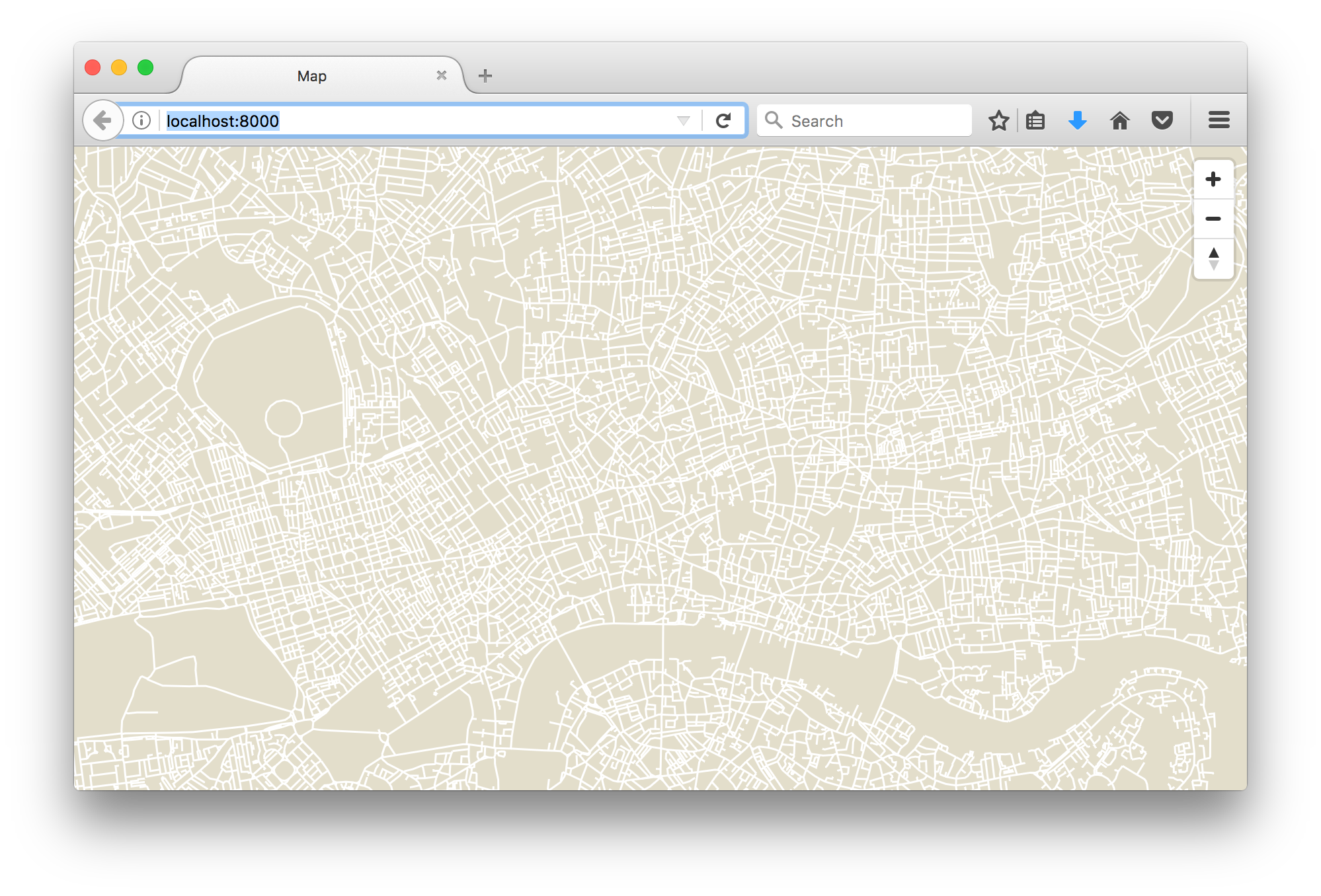
If you zoom out a bit you’ll see the extent of the data you’ve generated tiles for. Notice that all the roads are shown, but the individual road widths is thinner because of the styles you’ve set for each zoom range.
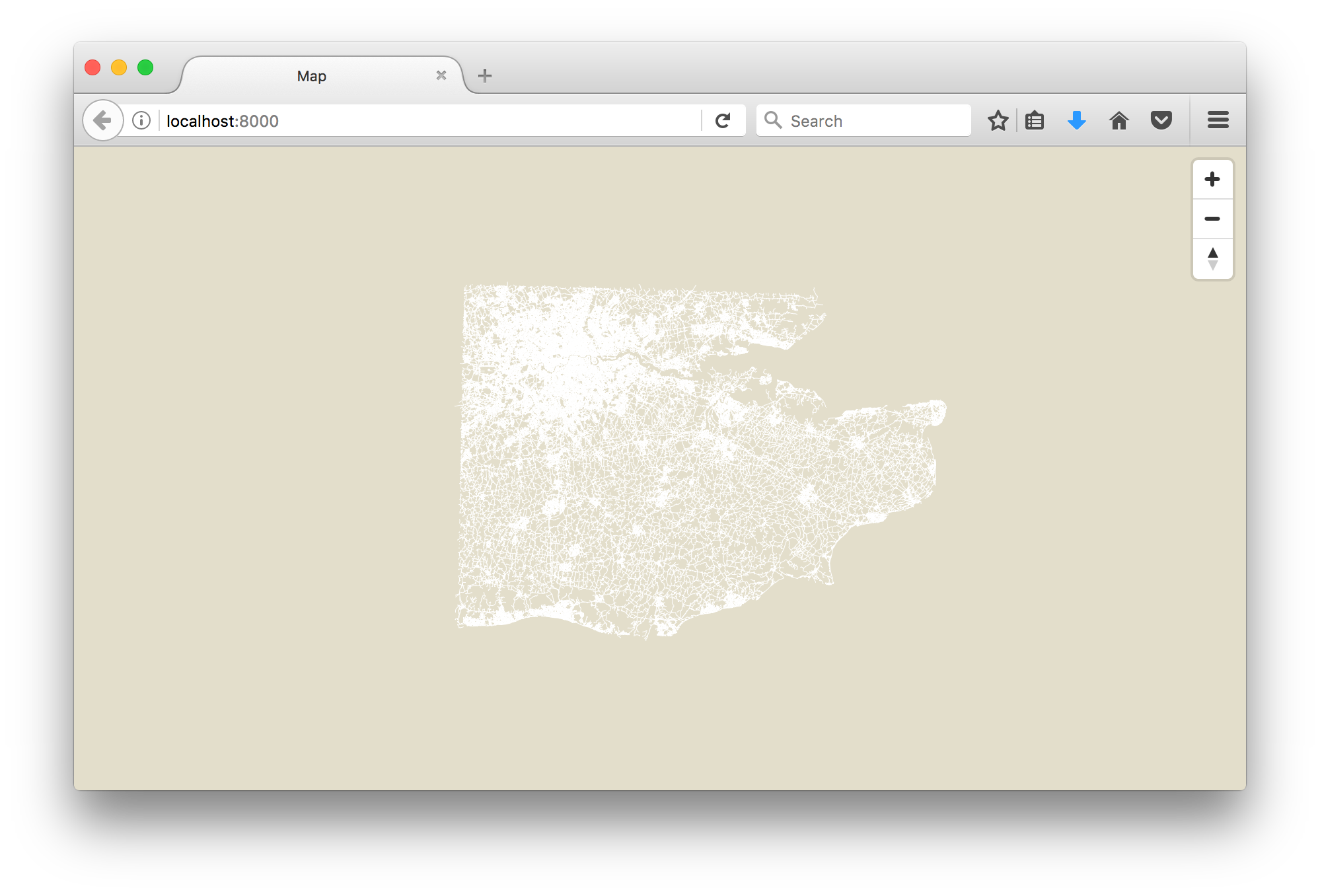
These screenshots contain OS Open Local data © Crown copyright and database right 2017
Advanced Styling Based on Attributes
Whilst changing styling based on zoom level is handy, it is also useful to be able to style the one vector tile layer in different ways according to the data it contains. In the case of roads, you might want main roads like A roads and motorways to be styled differently from B roads. You might want minor roads to only be visible when you are quite zoomed in.
You can achieve this with attributes and layer style filters.
When you ran tippecanoe you used the --exclude-all option to exclude all
the attribute data from the original shapefiles. This time, let’s use
--include to include just one attribute of the Road shapefile called
CLASSIFICA:
mv build/www/tiles build/www/tiles.old
time tippecanoe --no-feature-limit --no-tile-size-limit --include="CLASSIFICA" --maximum-zoom=16 --output-to-directory "build/www/tiles" `find ./build/geojson -type f | grep .json`
The tiles generated this time will include this extra data.
There is plenty of documntation on the OS Open Local data and in particular, the Product Guide pag 14 describes the Road attribute classifications:
- A Road
- B Road
- Local Road
- Local Access Road
- Restricted Local Access Road
- Minor Road
- Primary Road
- Motorway
- A Road, Collapsed Dual Carriageway
- B Road, Collapsed Dual Carriageway
- Minor, Collapsed Dual Carriageway
- Primary, Collapsed Dual Carriageway
- Motorway, Collapsed Dual Carriageway
- Shared use Carriageway
- Guided Busway Carriageway
ADVANCED TIP: There is a program called QGIS that you can install that helps
you work with shapefiles. If you drag the TQ_Roads.shp file into QGIS it will
draw all the roads for you. If you click the Open Attribute Table button
you’ll see a table of all the attribute data available, and the names of the
columns.
This means that now in the style layers, you can choose which features get styled by filtering only the features that have the attributes you want to style.
Here’s an example where we create three road style layers, each with a
different filter that uses the CLASSIFICA attribute. Note that some of the
style laters only show at certain zoom levels.
    {
      "id": "Road",
      "type": "line",
      "source": "composite",
      "source-layer": "Road",
      "minzoom": 12,
      "maxzoom": 15,
      "paint": {
          "line-color": "#FFFFFF",
          "line-width": 1.5
      },
      "filter": ["!in", "CLASSIFICA", "A Road", "A Road, Collapsed Dual Carriageway", "Motorway", "Primary Road", "Primary Road, Collapsed Dual Carriageway", "B Road"]
    },
    {
      "id": "MajorRoad",
      "type": "line",
      "source": "composite",
      "source-layer": "Road",
      "minzoom": 0,
      "maxzoom": 15,
      "paint": {
          "line-color": "#000000",
          "line-width": 3.5
      },
      "filter": ["in", "CLASSIFICA", "A Road", "A Road, Collapsed Dual Carriageway", "Motorway", "Primary Road", "Primary Road, Collapsed Dual Carriageway"]
    },
    {
      "id": "BRoad",
      "type": "line",
      "source": "composite",
      "source-layer": "Road",
      "minzoom": 0,
      "maxzoom": 15,
      "paint": {
          "line-color": "#888",
          "line-width": 1.8
      },
      "filter": ["in", "CLASSIFICA", "B Road", "B Road, Collapsed Dual Carriageway"]
    }
Summary
At this point you’ve successfully build a map using Vector Tiles that has different layers (roads and tidal water), and has different style layers for the road layer.
This is a great achievement! There’s still a lot more to learn about vector tiles including sprites, labels and simplification, but hopefully getting this far will have given you a great starting point for your explorations.
Feel free to leave questions or comments below and I’ll try my best to answer them.
Creative Commons Share-a-like James Gardner © Geovation

Leave a Comment